ModernBERT in Radiology Part 1: Simple Classifier using Hidden States
In Part 1 of the ModernBERT in Radiology series, we will explore ModernBERT and the ROCOv2 dataset for Radiology. We build a multi-label classifier using a simple Logistic Regression model on top of the pre-trained ModernBERT body.
You can follow along with the associated Colab Notebook for Part 1🔥!
The ModernBERT in Radiology Series
Part 1: Simple Classifier using Hidden States. 👈 This Post
Build a multi-label classification using a simple scikit-learn Logistic Regression model on top of the pre-trained ModernBERT body.
Part 2: Fine-tuning a Masked Language Model (MLM).
ModernBERT is pretrained as a Masked Language Model, but we perform a full fine-tuning using radiology text using
AutoModelForMaskedLM.Part 3: Fine-tuning for Classification.
Combining Part 1 and Part 2, we will build a ModernBERT classifier for the Part 1’s task, but perform a fine-tuning of the entire model using
AutoModelForSequenceClassification
We will be using the Hugging Face 🤗 transformers library and following some of the patterns shown in the excellent Natural Language Processing with Transforms book with code available on GitHub. Part 1 follows Chapter 2 of this book.

About ModernBERT
While LLMs like GPT-4, Claude, and Gemini are making all the news, these decoder-only models have cousins in the world of transformers: encoder-only models like BERT. While decoder-only can only see the tokens behind them (unidirectional attention, useful for text generation), encoder-only models can see the entire context (bidirectional attention), which can solve many traditional Natural Language Processing (NLP) tasks like classification, retrieval, and extraction. Encoder-only transformers are also faster than decoder-only transformers and can form the basis for techniques like Retrieval Augmented Generation (RAG) that can provide LLMs with additional relevant context.
Since BERT was released in 2018, there have been several successors, like RoBERTa. In December 2024, ModernBERT was announced. It increases the context length from 512 tokens to 8k, with a richer training data set and good performance characteristics. Read the Hugging Face article on ModernBERT for additional details.
Data
For speed of training, we’re going to use unsloth/Radiology_mini, which is a 0.33% sample from eltorio/ROCOv2-radiology. You would want to expand for a real model.
>>> dataset['train'][0]
{'image': <PIL.PngImagePlugin.PngImageFile image mode=L size=657x442>,
 'image_id': 'ROCOv2_2023_train_054311',
 'caption': 'Panoramic radiography shows an osteolytic lesion in the right posterior maxilla with resorption of the floor of the maxillary sinus (arrows).',
 'cui': ['C1306645', 'C0037303']}
The cui is a multi-label concept within the UMLS ontology. In this example, C1306645 is “Plain x-ray (C1306645)” and C0037303 is “Bone structure of cranium (C0037303)”. ROCOv2 has labeled the modality (e.g., “X-Ray” or “MRI”) and body part (e.g., “Abdomen”).
We are going to ignore the image and focus on caption and cui.
Note from eltorio/ROCOv2-radiology
The dataset labels and concepts were generated using the Medical Concept Annotation Toolkit v1.10.0 (MedCAT) and manually curated concepts for modality (all images), body region (X-ray only), and directionality (X-ray only).
Objective
We aim to train a model that can take in a caption and predict the CUIs.
Why this is interesting:
- ModernBERT has only been trained on the Masked Language task, not on a Classification task, which we are going to perform.
- We are going to leave ModernBERT’s pre-trained “body” in-place and replace the “head” (the final layer) with a custom classification layer, so we will be using ModernBERT’s last hidden network outputs as inputs to our simple classification model.
- We will be performing multi-label classification – each caption can have one or more
cuivalues.
For Part 1, we will create a simple scikit-learn Logistic Regression, which is ideal in CPU-only environments. In Part 3, we will do the same classification task, but with a Hugging Face-style transformer head using a Neural Net (NN) that we will save and compare to our Logistic Regression model.
WARNING Since the cui concepts were generated via MedCAT, we’re effectively going to be learning MedCAT’s predictions.
Code
See Colab for the full Notebook: https://colab.research.google.com/drive/1sfRbr-nE6LtJmgNFtOYstZ-YbIQ-DeMb?usp=sharing
Setup
In Part 1, we can run this on a Colab CPU. We use Hugging Face 🤗 transformers AutoModel to load the pre-trained ModernBERT since we will freeze the body and create a new head. If we did a full fine-tuning, we would use AutoModelForSequenceClassification instead.
pip install datasets evaluate wandb triton
pip install umap-learn
# Until next transformers release (4.48.0)
pip install git+https://github.com/huggingface/transformers.git
model_id = (
    "answerdotai/ModernBERT-base"
    # answerdotai/ModernBERT-large
)
dataset_name = (
    # "eltorio/ROCOv2-radiology"
    "unsloth/Radiology_mini" # 0.33% of ROCOv2-radiology, for a quicker demo
)

from transformers import AutoTokenizer, AutoModel
import torch

device = torch.device("cuda" if torch.cuda.is_available() else "cpu")
print(f"Using device: {device}")

tokenizer = AutoTokenizer.from_pretrained(model_id)
model = AutoModel.from_pretrained(model_id).to(device)
Load the Dataset
from datasets import load_dataset, DatasetDict
original_dataset = load_dataset(dataset_name)
Split the 15% of the total dataset from the train set into a validation set. We’ll hold back the test set for comparison between models.
Since we are not going to be interacting with the images, only the caption and cui, we will remove the image to save memory
validation_size = int(0.15 * (len(original_dataset['train']) + len(original_dataset['test'])))

dataset = DatasetDict({
    'train': original_dataset['train'].shuffle(seed=42).select(range(validation_size, len(original_dataset['train']))),
    'validation': original_dataset['train'].shuffle(seed=42).select(range(validation_size), )  ,
    # Keep the test -- we'll hold this back for comparison between models
    'test': original_dataset['test']
})

dataset = dataset.remove_columns(['image'])
I manually looked up the CUIs in this dataset, since UMLS Metathesauras requires a login. We will use it later only for some visualization, not for training.
cui_map = {
  'C0000726': 'Abdomen (C0000726)',
  'C0002978': 'angiogram (C0002978)',
  'C0006141': 'Breast (C0006141)',
  'C0023216': 'Lower Extremity (C0023216)',
  'C0024485': 'Magnetic Resonance Imaging (C0024485)',
  'C0030797': 'Pelvis (C0030797)',
  'C0032743': 'Positron-Emission Tomography (C0032743)',
  'C0037303': 'Bone structure of cranium (C0037303)',
  'C0037949': 'Vertebral column (C0037949)',
  'C0040405': 'X-Ray Computed Tomography (C0040405)',
  'C0041618': 'Ultrasonography (C0041618)',
  'C0205129': 'Sagittal (C0205129)',
  'C0817096': 'Chest (C0817096)',
  'C1140618': 'Upper Extremity (C1140618)',
  'C1306645': 'Plain x-ray (C1306645)',
  'C1996865': 'Postero-Anterior (C1996865)',
  'C1999039': 'Anterior-Posterior (C1999039)',
}
Tokenize the caption
AutoTokenizer will have loaded the pre-trained ModernBERT tokenizer. We need to make sure we use the same tokenizer!
We will use the tokenizer to add input_ids and attention_mask columns to the dataset.
def tokenize_function(examples):
    return tokenizer(
        examples["caption"],
        padding="max_length",
        truncation=True,
        # ModernBERT allows an increase to 8124 from 512 in BERT!
        # Our max len() of the captions in the train set is 934, so roughly 934/4 ~= 233,
        #  and further testing of the longest attention_mask shows this is actually 206.
        # Increasing too high will consume significant memory while we extract
        #  the hidden states for all the inputs.
        max_length=256,
      )

dataset = dataset.map(
    tokenize_function, batched=True
)
Convert cui to labels
Since this is a multi-label classification, we will use sklearn’s MultiLabelBinarizer , first fitting it to discover the classes, then applying those into a new labels column in the dataset.
from sklearn.preprocessing import MultiLabelBinarizer
import numpy as np
import pyarrow as pa

mlb = MultiLabelBinarizer()
train_labels = mlb.fit(dataset['train']['cui'])

def transform_labels(example):
    # Transform single example's CUIs to binary vector
    binary_labels = mlb.transform([example['cui']])[0]  # [0] to get the single example's labels

    example['labels'] = binary_labels.tolist()  # Convert numpy array to list for dataset storage
    example['num_labels'] = sum(binary_labels)

    return example

dataset = dataset.map(
    transform_labels,
    desc="Transforming labels to binary vectors",
    num_proc=4,
)
display(mlb.classes_)
# array(['C0000726', 'C0002978', 'C0006141', 'C0023216', 'C0024485',
#       'C0030797', 'C0032743', 'C0037303', 'C0037949', 'C0040405',
#       'C0041618', 'C0205129', 'C0817096', 'C1140618', 'C1306645',
#       'C1996865', 'C1999039', 'nan'], dtype=object)

display(dataset['train'][0]["labels"])
# [0, 0, 0, 0, 1, 0, 0, 0, 0, 0, 0, 0, 0, 0, 0, 0, 0, 0]
Explore ModernBERT’s last hidden layer
In Part 1, rather than fine-tuning a full model, we will lock the weights of the body of ModernBERT and use the hidden states of the last hidden layer as features for a small classifier model.
Let’s walk through one input to see the hidden layer outputs.
Our text here turns into a 14 token input:
text = "CT scan of brain and orbit showing thickened right optic nerve"
inputs = tokenizer(text, return_tensors="pt")
print(f"Input tensor shape: {inputs['input_ids'].size()}")
# Input tensor shape: torch.Size([1, 14])
inputs = {k:v.to(device) for k,v in inputs.items()}
with torch.no_grad():
    outputs = model(**inputs)
print(outputs)
# BaseModelOutput(last_hidden_state=tensor([[[ 1.0750, -1.3460, -0.8046,  ..., -0.6066,  0.2327, -0.6001],
#          [ 0.6414, -1.5472, -0.3777,  ..., -0.0761, -1.1976, -0.2748],
#          [ 0.4219, -2.2370, -0.7370,  ..., -1.3874, -2.0788, -0.2816],
#          ...,
#          [ 0.9101, -1.1216, -0.8162,  ..., -0.9774, -0.6886, -0.0127],
#          [-1.1381, -2.8003,  0.4157,  ..., -2.5451, -1.0654,  0.0358],
#          [ 0.3063, -0.1362,  0.0718,  ..., -0.0516,  0.0117, -0.2319]]],
#        device='cuda:0'), hidden_states=None, attentions=None)
A 768-dimensional vector is returned for each of the 15 input tokens
outputs.last_hidden_state.size()
# torch.Size([1, 14, 768])
def extract_hidden_states(batch):
    inputs = {k:v.to(device) for k,v in batch.items()
              if k in tokenizer.model_input_names}
    # Extract the last hidden states
    with torch.no_grad():
        last_hidden_state = model(**inputs).last_hidden_state
    # Return vector for [CLS] token
    return {"hidden_state": last_hidden_state[:,0].cpu().numpy()}

dataset.set_format(
    "torch",
    columns=["input_ids", "attention_mask", "labels"]
)

# If running out of memory, can reduce batch size, e.g. `batch_size=16`
hidden = dataset.map(extract_hidden_states, batched=True, batch_size=128)
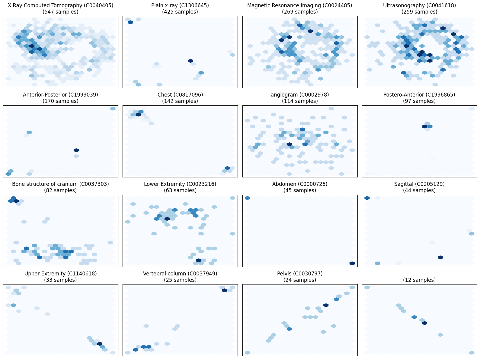
Visualize the Features
While not required to train a classifier, it would be helpful to visually check whether the hidden features are related to specific cui labels.
Let’s use UMAP to reduce the high-dimensional data. Visually, the hidden states seem differentiated.
Train a Logistic Regression Model
We are going to make a simple sklearn Logistic Regression model to take the hidden_states and predict one or more labels. Since we are doing a multi-label classification, we use OneVsRestClassifier
from sklearn.linear_model import LogisticRegression
from sklearn.multiclass import OneVsRestClassifier

classifier = OneVsRestClassifier(LogisticRegression(max_iter=1000))
classifier.fit(X_train, y_train)
The classifer accuracy at first does not look great, but we have an unbalanced multiclass dataset. We’ll look at correlations next.
classifier.score(X_valid, y_valid)
# 0.4608695652173913
Use the Classifier to Predict
Using the sklearn classifier, we can predict a few captions to get CUIs.
def predict(text):
  inputs = tokenizer(text, return_tensors="pt")
  inputs = {k:v.to(device) for k,v in inputs.items()}
  with torch.no_grad():
      outputs = model(**inputs)
  hidden_state = outputs.last_hidden_state[:,0].cpu().numpy()
  prediction = classifier.predict(hidden_state)

  # get the labels
  predicted_labels = mlb.inverse_transform(prediction)[0]

  print(f"{text}: {[cui_map.get(label) for label in predicted_labels]}")

predict("CT of Chest with pneumothorax")
# CT of Chest with pneumothorax: ['X-Ray Computed Tomography (C0040405)']
predict("Abdomen x-ray with small bowel obstruction")
# Abdomen x-ray with small bowel obstruction: ['Abdomen (C0000726)', 'Plain x-ray (C1306645)']
That looks pretty good.
Correlation of multi-label classification
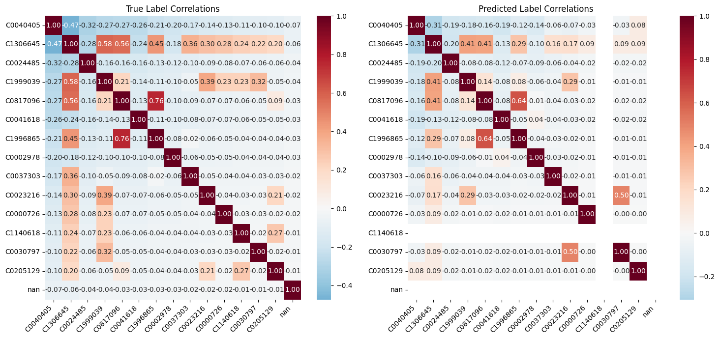
We do see an overlap between Chest (C0817096) and Postero-Anterior (C1996865), but that is expected since those are often overlapping labels.
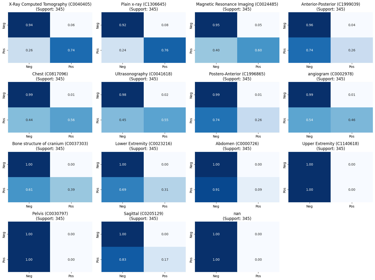
We can also look at per-label confusion matrices.
Next Steps
Follow along for the next posts in the series:
- Part 2: Fine-tuning a Masked Language Model (MLM)
- Part 3: Fine-tuning for Classification. Coming Soon
Subscribe to get notified when the next Parts of the ModernBERT in Radiology series are published.
Read more about ModernBERT:
- https://huggingface.co/answerdotai/ModernBERT-base
- https://huggingface.co/blog/modernbert
- https://github.com/nlp-with-transformers/notebooks
Citations
- Warner, B., Chaffin, A., Clavié, B., Weller, O., Hallström, O., Taghadouini, S., Gallagher, A., Biswas, R., Ladhak, F., Aarsen, T., Cooper, N., Adams, G., Howard, J., & Poli, I. (2024). Smarter, Better, Faster, Longer: A Modern Bidirectional Encoder for Fast, Memory Efficient, and Long Context Finetuning and Inference. arXiv preprint arXiv:2412.13663.
- Ronan, L. M. (2024). ROCOv2-radiology [Dataset]. Hugging Face. https://doi.org/10.57967/hf/3489
- Tunstall, L. (2022). Natural Language Processing with Transformers: Building Language Applications with Hugging Face. O’Reilly Media.